A quick-start guide to the `caret` R package
Background
The caret R package has been a staple of machine learning (ML) methods in R for a long time. The name caret stands for “Classification and Regression Training” according to the authors. It provides methods for common ML steps, such as pre-processing, training, tuning, and evaluating predictive models.
In addition to caret, there is also a group of packages referred to as tidymodels that is currently in development and which is also available for use. Both caret and tidymodels have Max Kuhn as a main author, but tidymodels aims to streamline ML for use with tidyverse packages.
I’ll be focusing on caret in this intro. We’ll be working with data from the palmerpenguins package, and using the caret, and tidyverse packages.
Working with data
Start by loading the necessary packages:
library(tidyverse)
library(palmerpenguins)
library(caret)
We’ll use the penguins dataset from palmerpenguins. It will be loaded automatically when you load the palmerpenguins package:
head(penguins)
| species | island | bill_length_mm | bill_depth_mm | flipper_length_mm | body_mass_g | sex | year |
|---|---|---|---|---|---|---|---|
| Adelie | Torgersen | 39.1 | 18.7 | 181 | 3750 | male | 2007 |
| Adelie | Torgersen | 39.5 | 17.4 | 186 | 3800 | female | 2007 |
| Adelie | Torgersen | 40.3 | 18.0 | 195 | 3250 | female | 2007 |
| Adelie | Torgersen | NA | NA | NA | NA | NA | 2007 |
| Adelie | Torgersen | 36.7 | 19.3 | 193 | 3450 | female | 2007 |
| Adelie | Torgersen | 39.3 | 20.6 | 190 | 3650 | male | 2007 |
This package contains LTER data for three penguin species on islands in Antarctica.
Reviewing the data
caret provides a function called featurePlot(), which is used to visualize datasets. It runs off of the lattice package, so if you are familiar with this method of plotting you might find it familiar. As someone who primarily uses ggplot2 I found this function a bit difficult to use, but you may find it helpful still. Max Kuhn’s The caret` Package Bookdown document provides some interesting examples of its functionality. Here’s a basic plot with a couple of our variables:
featurePlot(x = penguins[, c("bill_length_mm", "bill_depth_mm", "flipper_length_mm")],
            y = penguins$body_mass_g,
            plot = "scatter",
            layout = c(3, 1))
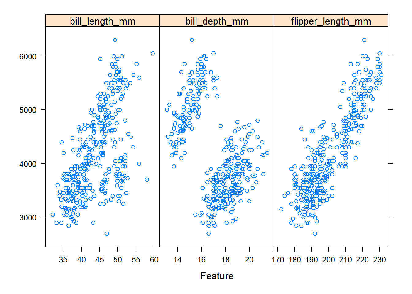
In the plot above, the x-axis corresponds to each predictor (by panel) and the y-axis is body_mass_g.
Pre-processing
caret has built-in functionality to help with pre-processing your data as well. There are some more sophisticated options, but here we’ll just take a look at one. For example, in some modeling situations you’ll want to check for correlated predictors (multicollinearity). The caret function for this is findCorrelation().
First we’ll want to make a correlation matrix, which will be fed into findCorrelation().
penguin_cor <- penguins %>%
  filter(!if_any(everything(), is.na)) %>%
  # Numeric columns only
  select(where(is.numeric)) %>%
  cor()
Then findCorrelation() will check for correlations above a cutoff value that we provide:
findCorrelation(x = penguin_cor,
                # Use 0.7 correlation cutoff
                cutoff = 0.7,
                # Provide more details
                verbose = TRUE,
                # Return column names instead of indices
                names = TRUE)
## Compare row 3  and column  4 with corr  0.873
##   Means:  0.564 vs 0.334 so flagging column 3
## All correlations <= 0.7
## [1] "flipper_length_mm"
It notes that row 3 and column 4 of our correlation object have a correlation of 0.87:
##                   bill_length_mm bill_depth_mm flipper_length_mm body_mass_g
## bill_length_mm         1.0000000    -0.2286256         0.6530956  0.58945111
## bill_depth_mm         -0.2286256     1.0000000        -0.5777917 -0.47201566
## flipper_length_mm      0.6530956    -0.5777917         1.0000000  0.87297890
## body_mass_g            0.5894511    -0.4720157         0.8729789  1.00000000
## year                   0.0326569    -0.0481816         0.1510679  0.02186213
##                          year
## bill_length_mm     0.03265690
## bill_depth_mm     -0.04818160
## flipper_length_mm  0.15106792
## body_mass_g        0.02186213
## year               1.00000000
This means flipper_length_mm (row 3) and body_mass_g (column 4) are correlated. That’s fine since body mass is our response variable.
Splitting the data
We’ll want to make a training dataset with which to build our model. caret provides some methods for doing this, including some for balanced splits for classification datasets, splitting using maximum dissimilarity, splitting for time series, and more.
We’ll proceed by modeling body_mass_g. First we’ll remove NAs, then do a basic split into a training dataset.
model_data <- penguins %>%
  filter(!if_any(everything(), is.na))

# 80% of the data for training - these are row indices
set.seed(500)

training_indices <- createDataPartition(y = model_data$body_mass_g,
                                        p = .8,
                                        # Do not return a list
                                        list = FALSE)

# Subset the rows selected above
training_sample <- model_data[training_indices, ]
Modeling
With our data in hand we now can progress to training a model. We’ll use a random forest for this example. Note that there is a lot to explore in caret that I won’t go over here. I highly recommend reading The caret` Package.
First we can use the trainControl() function to customize the model training process:
train_params <- trainControl(
  # Repeated K-fold cross-validation
  method = "repeatedcv",
  # 10 folds
  number = 10,
  # 3 repeats
  repeats = 3
)
Now we can train the random forest with the parameters above:
set.seed(500)

rf_model <- train(
  # Modeling formula indicating to model body_mass_g using all other vars
  form = body_mass_g ~ .,
  # Our custom parameters
  trControl = train_params,
  # The dataset
  data = training_sample,
  # Use a random forest
  method = "rf"
)
Here are our results:
# Note that mtry = the number of randomly selected predictors caret uses at each split
rf_model
## Random Forest
##
## 268 samples
## 7 predictor
##
## No pre-processing
## Resampling: Cross-Validated (10 fold, repeated 3 times)
## Summary of sample sizes: 242, 241, 242, 241, 241, 242, ...
## Resampling results across tuning parameters:
##
## mtry RMSE Rsquared MAE
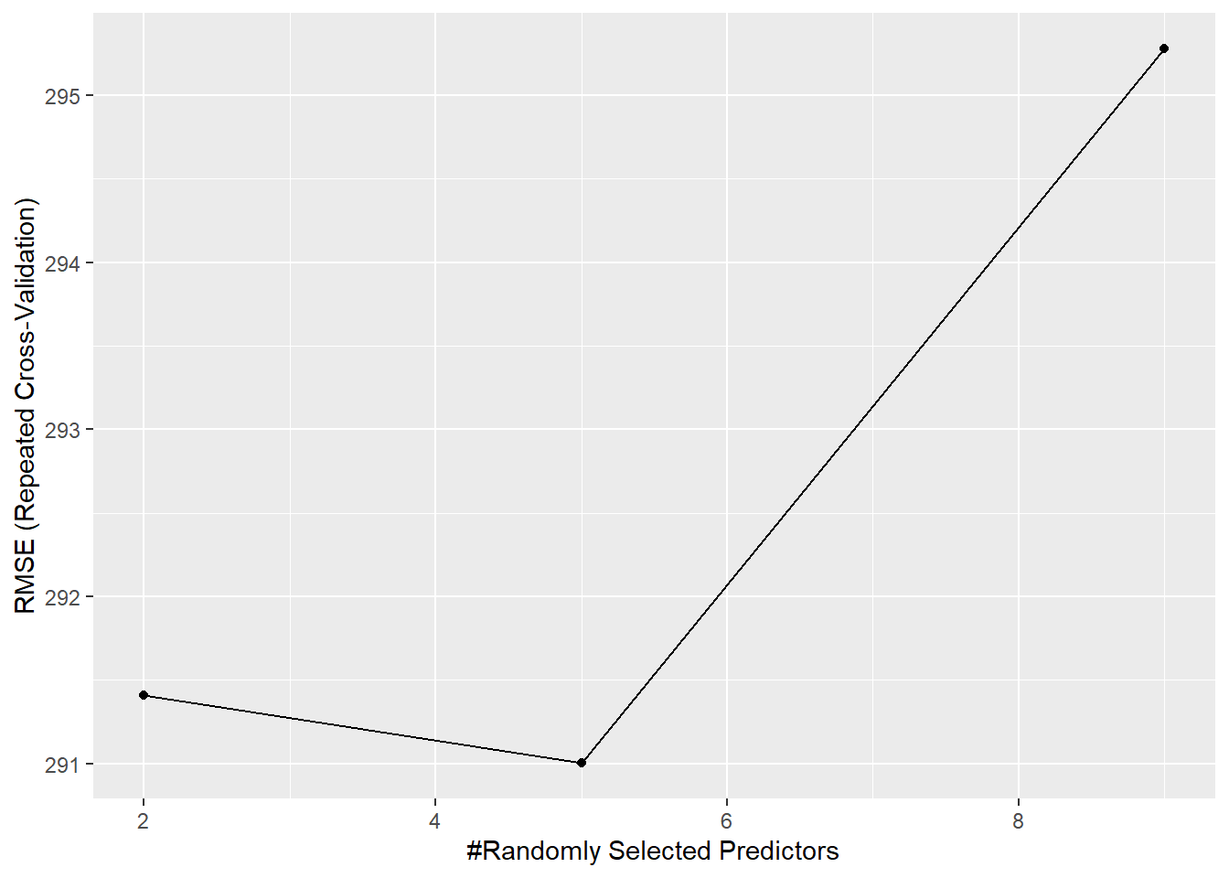
## 2 291.4107 0.8760304 233.9042
## 5 291.0023 0.8739321 234.9932
## 9 295.2779 0.8700284 240.0389
##
## RMSE was used to select the optimal model using the smallest value.
## The final value used for the model was mtry = 5.
The final model can be accessed from the trained object. But note that you probably shouldn’t rely on this R^2^ as your output.
rf_model$finalModel
##
## Call:
##  randomForest(x = x, y = y, mtry = min(param$mtry, ncol(x)))
##                Type of random forest: regression
##                      Number of trees: 500
## No. of variables tried at each split: 5
##
##           Mean of squared residuals: 86096.17
##                     % Var explained: 86.69
Its mtry value was 5 based on RMSE, which we can view using ggplot():
ggplot(rf_model)
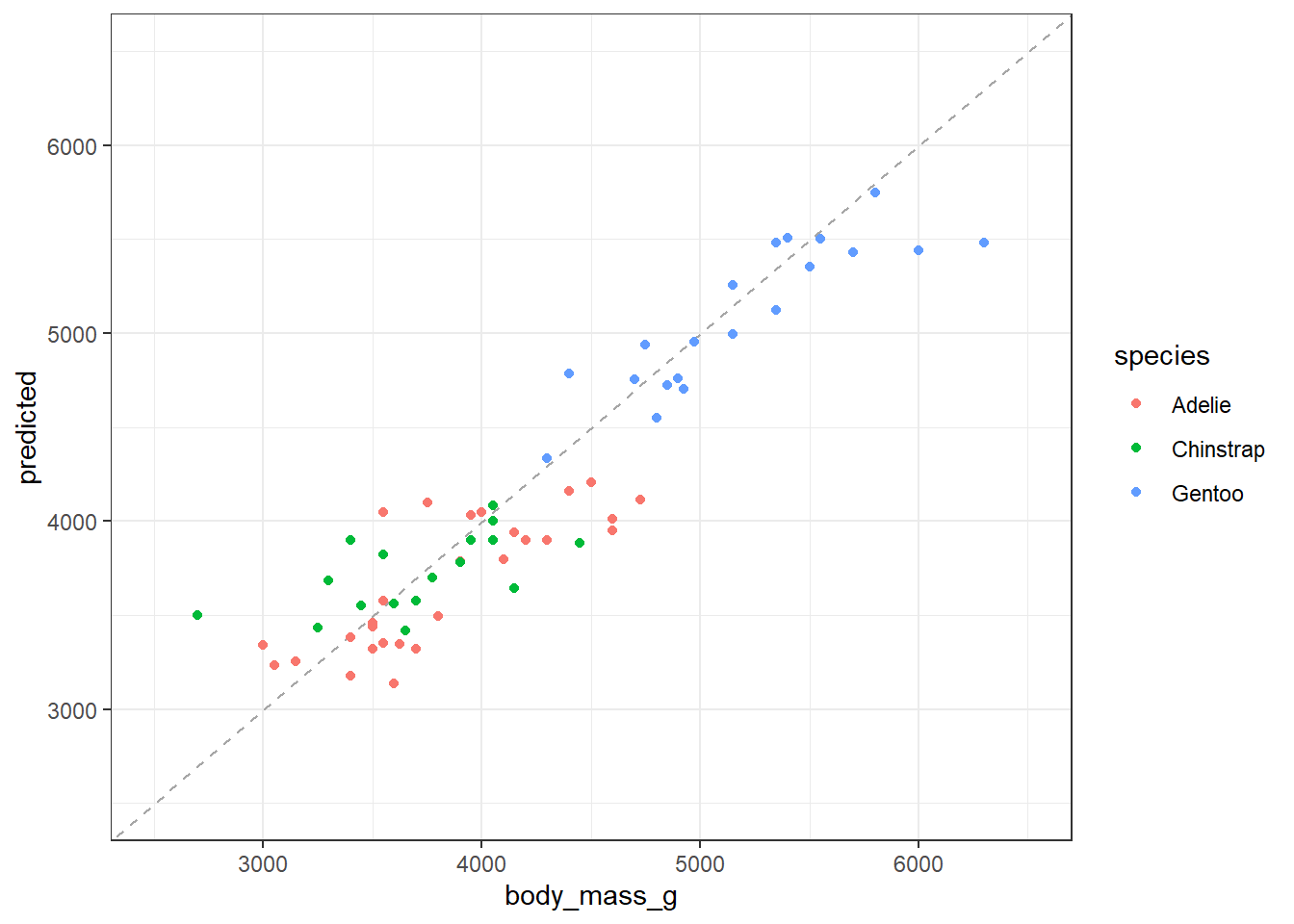
Now we want to know how the model performs on our testing data subset:
# Pull out the rows for testing and add predictions from the RF
test_sample <- model_data[-training_indices, ] %>%
  mutate(predicted = predict(object = rf_model, newdata = .))

# Get a new R2
postResample(pred = test_sample$predicted,
             obs = test_sample$body_mass_g)
##       RMSE   Rsquared        MAE
## 310.377285   0.864062 241.696781
Plot the relationship
ggplot(data = test_sample) +
  # A 1:1 line
  geom_abline(slope = 1, intercept = 0, linetype = "dashed", color = "gray65") +
  geom_point(aes(x = body_mass_g, y = predicted, color = species)) +
  xlim(c(2500, 6500)) +
  ylim(c(2500, 6500)) +
  theme_bw()
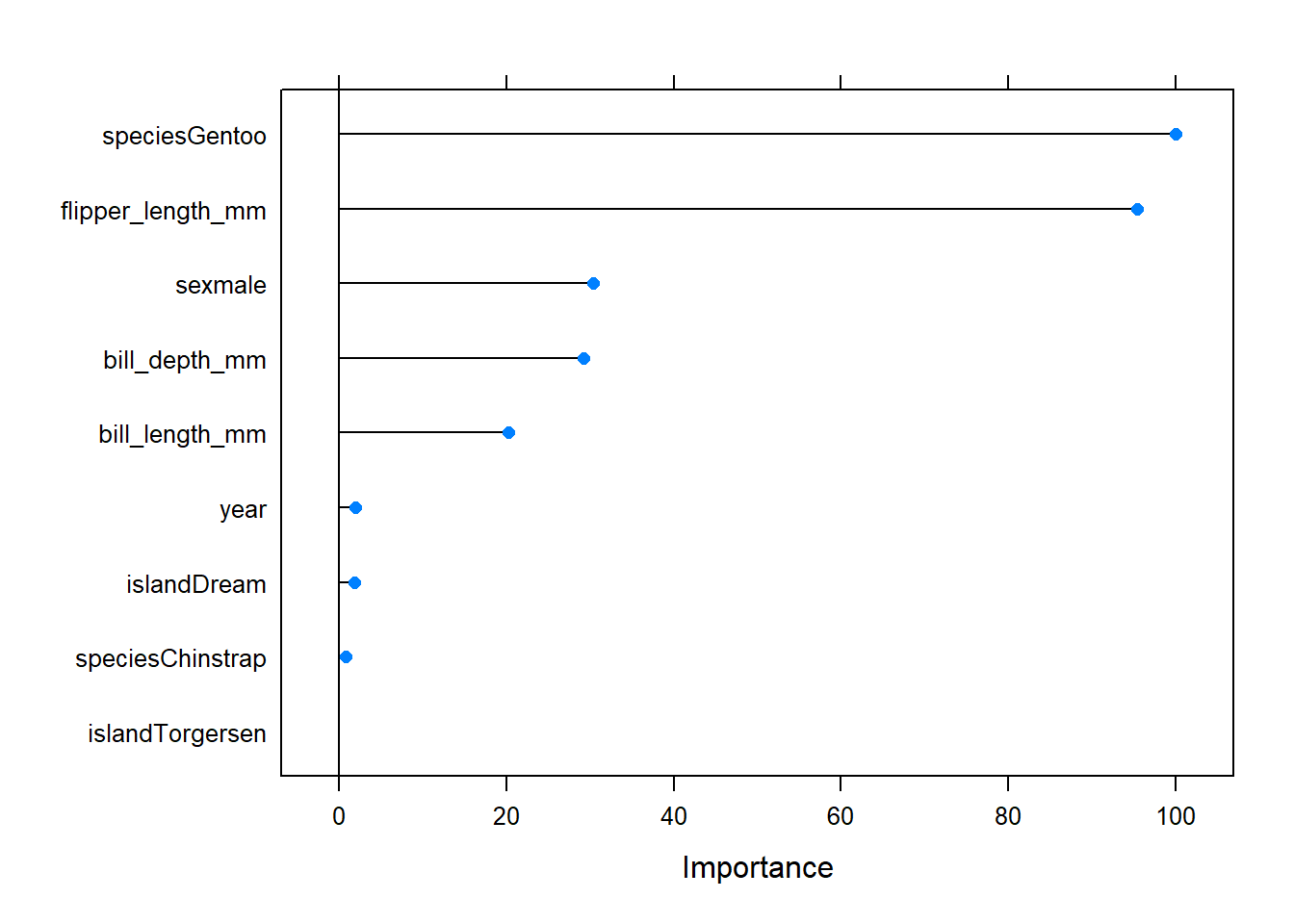
We can look at a scaled metric for variable importance using the varImp() function:
plot(varImp(rf_model))